
Results
Schools differ in how many organizations they work with
Schools differ mainly in how many of the seven organizations they work with: civic groups, local businesses, churches, social services, mental-health providers, juvenile justice agencies and the police. The particular ones a school picks are close to unpredictable. Knowing the count barely narrows them down, and nothing else the survey records narrows them either: not the size of the school, not its grade level, not whether it is in a city or the countryside, not the make-up of its student body.
A statistical model of the whole network says the same thing. The uneven spread of ties across schools comes out at -0.885, and the minus sign means some schools hold far more ties than chance would give them. Schools vary far more than they would if each relationship were decided on its own.
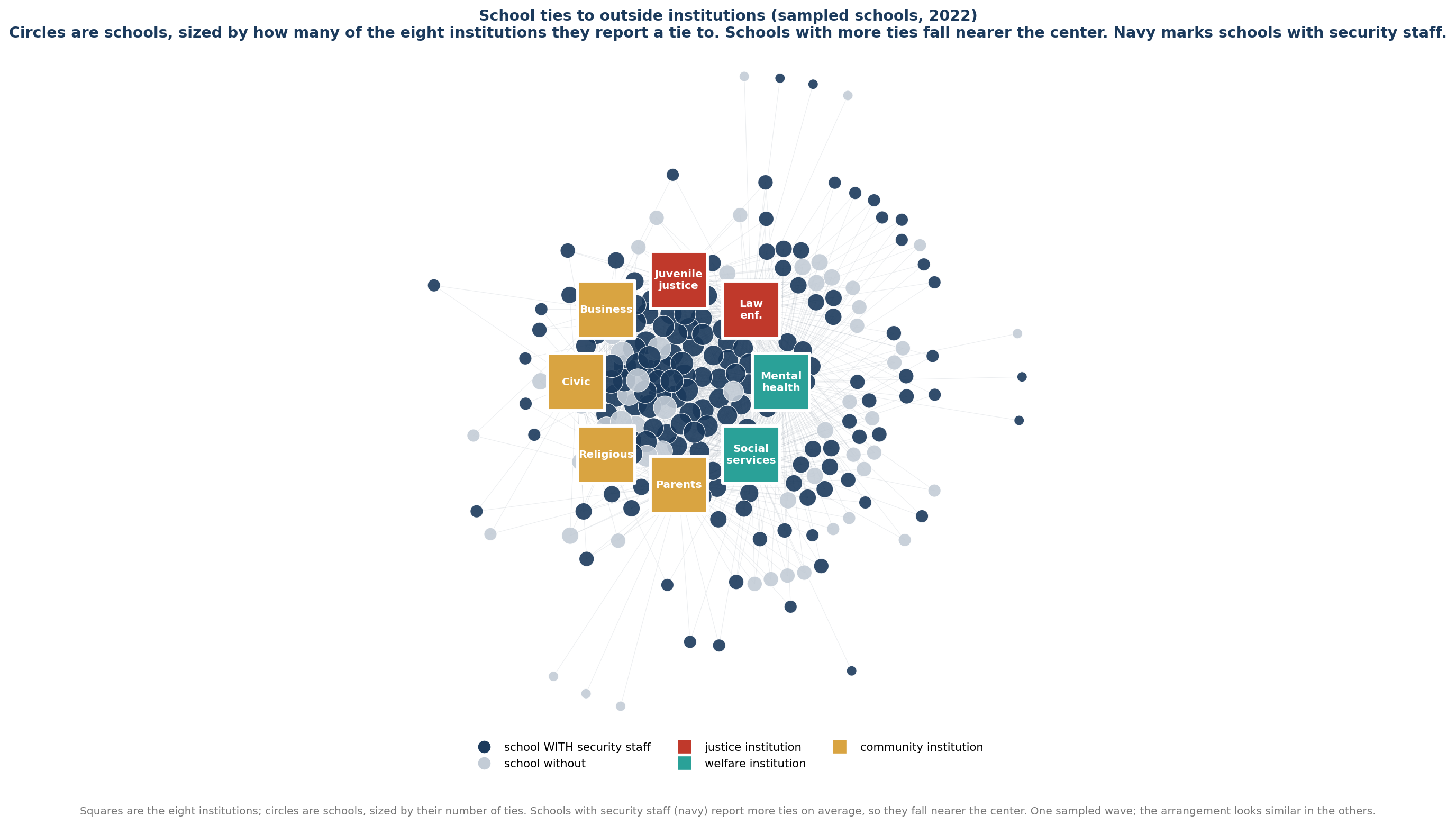
Table 2. A network model of which schools work with which of the seven organizations, fitted to the 2015-16 survey (n = 1,726 schools)source table 1
| (1) The neighborhood on its own | (2) Adding what the school runs | (3) Asking which organization | |
|---|---|---|---|
| Shape of the network | |||
| Baseline rate at which schools and organizations are tied (edges) how dense the network is overall, like an intercept |
+0.126 (0.022)*** | -0.092 (0.041)* | -1.208 (0.069)*** |
| How unevenly ties are spread across schools (gwb1degree, decay 0.4) negative means some schools hold far more ties than chance would give |
-1.093 (0.133)*** | -0.885 (0.147)*** | -2.031 (0.141)*** |
| What the school is dealing with | |||
| Recorded incidents of crime and violence standardized |
+0.062 (0.021)** | +0.068 (0.022)** | |
| Crime level the principal reports for the area standardized; higher means more crime. This is the principal's description, not a recorded crime count |
+0.041 (0.017)* | -0.001 (0.018) | +0.036 (0.020) |
| What the school is | |||
| Size of the school standardized |
+0.105 (0.017)*** | +0.026 (0.020) | +0.029 (0.021) |
| Inadequate funds limit crime prevention | -0.004 (0.016) | +0.002 (0.017) | +0.001 (0.018) |
| What the school runs for itself | |||
| Employs security staff guards, resource officers or sworn police |
+0.272 (0.042)*** | +0.295 (0.046)*** | |
| Formal process for consulting parents standardized; includes training or services offered to parents |
+0.138 (0.018)*** | +0.150 (0.019)*** | |
| Which organization, not how many | |||
| The crime level the principal reports, on the police tie only an edge covariate carrying the school's standardized reading on the police column and zero elsewhere, so the coefficient is how much more or less the police tie answers to that reading than the average organization does |
-0.335 (0.069)*** | ||
| A separate baseline for each organization so that the police being the commonest tie is a main effect rather than something the row above has to carry |
no | no | yes |
Note: A coefficient is the change in the log odds of a school working with a given organization. The first two terms describe the shape of the network. The rest ask whether schools with more of that characteristic hold more ties, which this kind of model calls an activity effect, so columns 1 and 2 speak to how many ties a school holds and not to which. Column 1 puts the neighborhood in on its own; column 2 adds the three things the school runs for itself, and the neighborhood coefficient falls to nothing, which is the paper's direct-and-indirect result inside the model. Column 3 asks the compositional question instead. With every organization given its own baseline, and the degree term already holding how concentrated the ties are, the edge covariate is the police tie's own answer to the neighborhood reading, at -0.335 against a general activity effect of +0.036 in the same model. That is the fixed-count result of Table 18 estimated inside the two-mode model rather than beside it. Checked with an estimator that shares nothing with it: laying the same schools out as 12,082 school-and-organization pairs and giving every school its own intercept, which removes that school's count of partners from the comparison altogether, the crime reading predicts the police cell at -0.046***, against the other cells of the same row. Unweighted, since exponential random graph models do not take survey weights. ***p < 0.001, **p < 0.01, *p < 0.05.
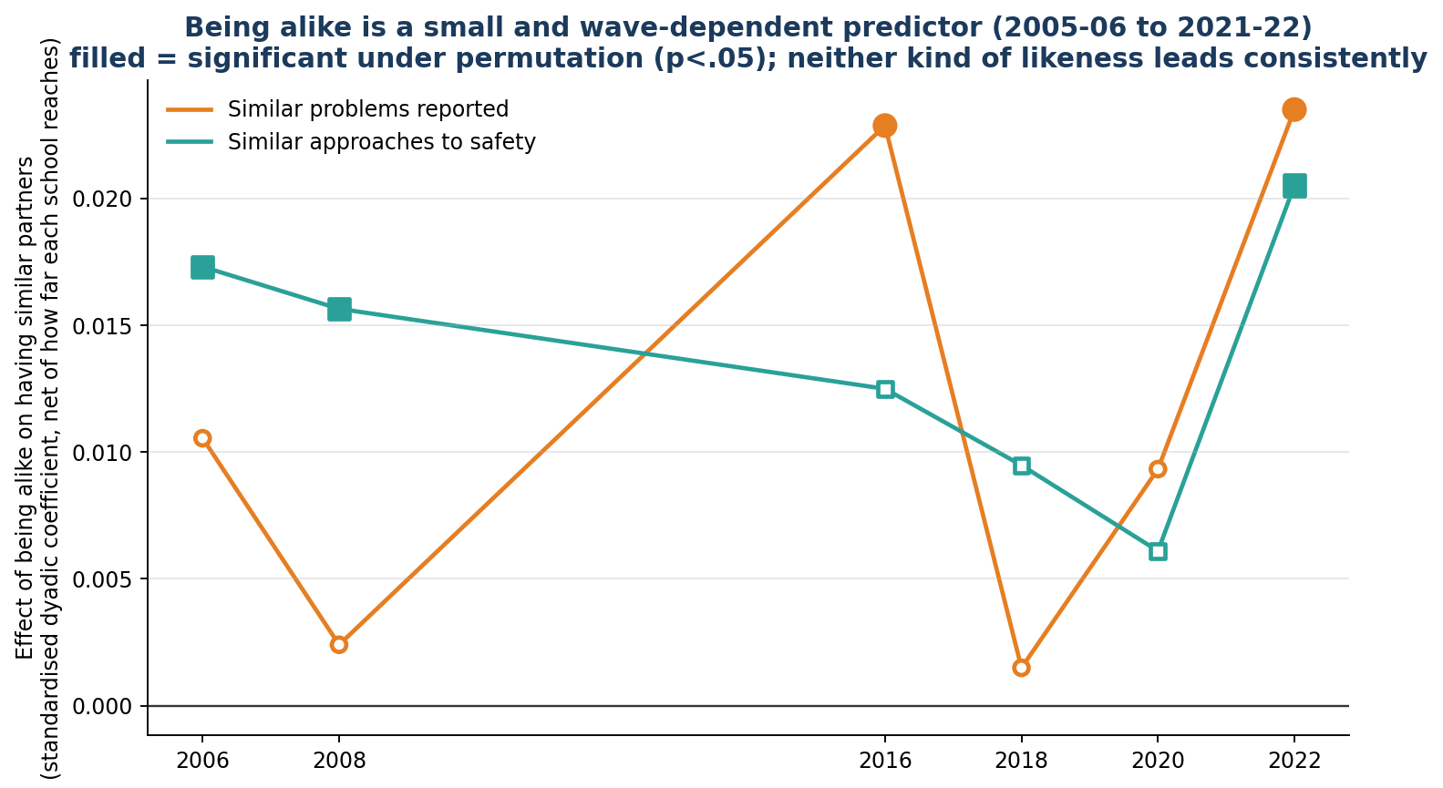
One faint pattern does survive. Among the seven organizations, three pairs turn up together slightly more often than chance: social services with mental-health providers, juvenile justice agencies with the police, and civic groups with local businesses. The effect is small, and it sorts the organizations rather than the schools, so the finding that schools have no types still stands.
Table 3. How often the seven organizations turn up together, against 300 reshuffles that keep every school's number of organizations and every organization's popularity exactly as observed, by surveysource table 19
| Wave | Within-side co-occurrence, z | Social services with mental health, z | Juvenile justice with the police, z | Civic groups with businesses, z |
|---|---|---|---|---|
| 2005-06 | 18.6 | 8.2 | 8.8 | 10.2 |
| 2007-08 | 16.3 | 7.6 | 7.8 | 7.9 |
| 2015-16 | 12.5 | 8.8 | 6.0 | 5.9 |
| 2017-18 | 17.3 | 7.2 | 4.5 | 9.4 |
| 2019-20 | 14.1 | 5.0 | 5.6 | 7.5 |
| 2021-22 | 14.6 | 6.4 | 4.7 | 6.9 |
Note: Each z compares the observed number of schools holding both ties in a pair (summed over the nine within-side pairs in the first column, single pairs in the others) against 300 curveball randomizations that hold every school's count of ties and every organization's prevalence exactly fixed, so the margins explain none of it. The structure is present in every wave and it is small: the first two eigenvalues of the tetrachoric correlation matrix are 2.4 and 1.5, so the count's dimension is about 1.6 times the size of the sides dimension, and at a fixed count the residual correlations of the three pairs shown are -0.04, +0.06, +0.05 against a compositional baseline of -0.17, the mean over all 21 pairs. A varimax rotation of the two factors reproduces the community and government sides used throughout the paper. Randomization seed 7; reproduce.R rechecks the observed totals exactly and the z-scores with independent draws.
These numbers cover the 12,691 school responses that work with between one and six of the seven. The 2,504 that work with all seven or with none are set aside. Putting them back raises the main estimate from +0.104 to +0.129. Schools land in that set-aside group at about the same rate whatever the principal says about crime: 16.8% where the area is called low-crime, 16.8% where it is called moderate and 15.1% where it is called high-crime.
Security staff, parent processes and equipment predict most
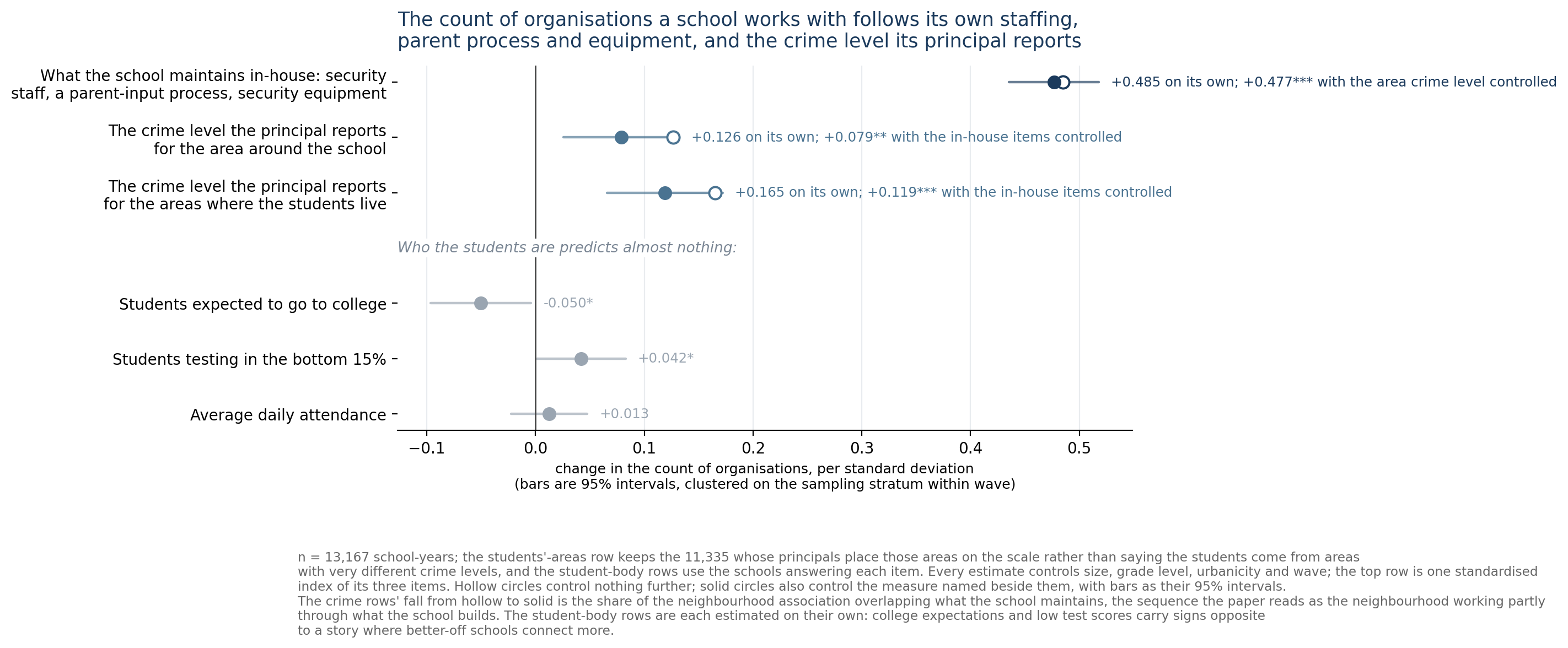
Schools that have security staff, a formal process for consulting parents, and security equipment work with more outside organizations. This is the strongest pattern in the data. Two schools one standard deviation apart on those three differ by about +0.377 of an organization out of the seven, a little under two fifths of one.
It holds in all six surveys, from +0.343 in 2005-06 to +0.428 in 2019-20. Drop any single survey and the overall figure stays between +0.362 and +0.392. It holds at every grade level too: +0.42 in primary schools, +0.32 in middle schools and +0.26 in high schools.
You might worry that this is circular, because security staff can include police officers and one of the seven organizations is the police. It is not. Leave out the police and count only the other six, and the figure is +0.334, the same rate per organization.
Those three measure how much a school runs, not which kind of organization it favors. Among schools with the same number of partners, security staffing leans slightly towards the government organizations (+0.048), and the parent process (-0.034) and security equipment (-0.034) lean slightly towards the community ones.
Table 6. Security staff, the parent process and equipment, and the crime level the principal reports, entered alone and entered togethersource table 17
| Entered alone | Entered together | |
|---|---|---|
| What the school has built (staff, parent process, equipment) | +0.384*** (0.020) | +0.377*** (0.020) |
| How its principal reads the environment | +0.104*** (0.024) | +0.067** (0.023) |
| The two multiplied | -0.028 (0.015) | |
| Inadequate funds limit crime prevention: a little (against not at all) | +0.222*** (0.043) | +0.210*** (0.043) |
| Inadequate funds limit crime prevention: a lot (against not at all) | +0.138** (0.044) | +0.132** (0.044) |
| ...the reading of where the students live (10,927 school-years; entered with capacity in the second column) | +0.152*** (0.024) | +0.116*** (0.023) |
| Does advantage build reach? | ||
| Share of students expected to go to college | -0.067** (0.021) | -0.057** (0.022) |
| Share testing in the bottom fifteen per cent | +0.054** (0.019) | +0.039* (0.020) |
| Average daily attendance | +0.018 (0.016) | +0.027 (0.015) |
Note: n = 12,691. Survey-weighted, standard errors clustered on the sampling stratum within wave, in brackets. All predictors standardized, so each coefficient is the difference in the count of organizations between two schools one standard deviation apart. What the school has built is an index of the three standing arrangements the survey carries in every wave: security staffing (harmonized to any-versus-none across a wording change in 2015-16), the formal parent process, and security equipment; each is standardized, the three are averaged, and the average is restandardized. Every model controls for size, grade level, urbanicity, wave and how far inadequate funds limit the school's crime prevention; the within-wave estimates drop the wave. The capacity coefficient carries the scrutiny the environmental one does. Estimated within wave it is 2005-06 +0.343***, 2007-08 +0.396***, 2015-16 +0.350***, 2017-18 +0.350***, 2019-20 +0.428***, 2021-22 +0.374***, significant in all six; leaving any one wave out keeps the pooled estimate between +0.362 and +0.392. It is not an artefact of overlap between the index and the ties (the staffing measure includes sworn officers; one tie is law enforcement): on the six ties excluding the police it is +0.334*** (0.020), the same rate per organization. The index measures how much machinery, not which kind: at a fixed count, security staffing goes with the government side of the field (+0.048**) and the parent process with the community side (-0.034*), while equipment goes with the community side (-0.034*). In the joint rows the two main effects come from the additive model; the product row comes from the model that adds it, whose main effects are +0.379 and +0.066. The interaction implies an environmental slope of +0.094 (0.027)*** at -1, +0.066 (0.023)** at +0, +0.037 (0.028) at +1, +0.009 (0.039) at +2 standard deviations of capacity: the first two separate from zero and the last two do not, so the environmental route is clear at and below average capacity and cannot be distinguished from zero in the sixth of schools more than one standard deviation above it. The last three rows test whether advantage builds reach. Entered alone, the share expected to go to college and the share testing at the bottom carry the wrong sign for a position account; entered together both keep those signs and still separate from zero, at -0.057** and +0.039*, and with the crime reading and all five student-body measures present they are -0.038 and +0.019. Nothing here suggests that advantage builds reach. The funding rows compare schools whose principals say inadequate funds limit their crime prevention a little or a lot with schools saying not at all. Estimated within each crime reading, with the standard controls, they are low crime (9,488 school-years) +0.209*** and +0.101*; moderate crime (2,460 school-years) +0.230* and +0.093; high crime (743 school-years) +0.195 and +0.223. ***p < 0.001, **p < 0.01, *p < 0.05.
How the principal describes the neighborhood
The survey asks principals to describe the crime level in the area around the school as low, moderate or high. Schools whose principals say high work with more outside organizations. The average school called low-crime works with 3.34 of the seven and the average school called high-crime with 3.62, a gap of a little over a quarter of one organization, on a count that averages 3.40. Among schools of the same size, grade level, city or rural location and survey year, where funding limits crime prevention to the same degree, the difference is +0.104 of an organization per standard deviation of the crime rating. It shrinks to +0.067 once the school's own staff, parent process and equipment are accounted for, and it is still there.
This is where the two research traditions set out under Theory can be told apart. Resource dependence reads a wide network as a sign of an organization under pressure, and predicts this. Social capital as Nan Lin sets it out predicts the opposite, because it reads a wide network as a sign of an organization doing well.
The effect is not the same in every survey. Pooled across all six it is +0.104, but a test says the surveys genuinely differ from each other rather than wobbling by chance (F = 4.13, p = 0.0012). So treat +0.104 as an average over six years that differ, not as one stable number.
Does the principal's answer mean anything?
The crime level in this study is not a police statistic. It is one thing a principal typed into a form. Asked how much crime there is in the area around the school, they picked low, moderate or high.
That is worth stopping on. If the answer were just a mood, or a habit of speech, this study would be about how principals talk rather than about where schools are.
So we checked it against three measures the study never uses it to predict.
Schools whose principals report more crime have more crimes actually recorded against them that year, at +0.103. The survey counts those in a separate set of questions about what happened at the school.
Staff at those schools report more bullying, harassment and verbal abuse, at +0.154.
And fewer parents turn up to school events, at -0.185, the largest of the three in size. That covers open houses, parent-teacher meetings, subject evenings and volunteering.
None of those three is one of the seven organizations, and none of them is used anywhere else in this study. So a principal who says the area is rough is describing a school with more recorded crime, more trouble reported by staff, and fewer parents coming through the door.
That does not turn the answer into a measurement. It is still what one person thought, and two principals looking at the same streets could answer differently. The three checks settle one point only: the answer is not cut off from what happens at the school.
Which organizations schools in rougher areas add
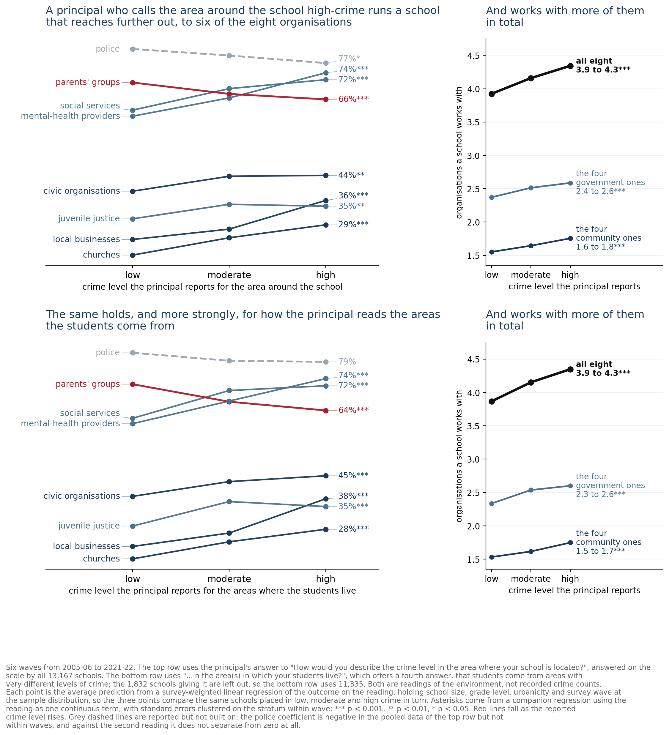
When a school in a high-crime area works with more organizations, the extra ones are spread across community groups and government agencies alike. They are not concentrated on the police and the courts. The count of community partners and the count of government partners both rise by about the same amount, and the balance between the two sides does not change.
Six of the seven come out higher as the reported crime level rises, once school size, grade level, where the school is and which survey are allowed for, along with how far a lack of funds limits the school's crime prevention. The biggest rise is for mental-health providers, at +0.029 per standard deviation. Social services and local businesses each rise by +0.024, churches by +0.023 and civic groups by +0.013. Juvenile justice agencies rise by +0.011, which does not separate from zero. The police fall instead, at -0.020, and the next section is about them.
Table 13. Each of the seven organizations against the crime level the principal reportssource table 4
| Organization | Side | Coefficient | Clustered SE | Share of schools with the tie |
|---|---|---|---|---|
| Civic organizations | community | +0.013* | 0.006 | 42% |
| Local businesses | community | +0.024*** | 0.006 | 27% |
| Churches | community | +0.023*** | 0.006 | 22% |
| Social services | government | +0.024*** | 0.006 | 68% |
| Mental-health providers | government | +0.029*** | 0.007 | 66% |
| Juvenile justice | government | +0.011 | 0.006 | 33% |
| Police | government | -0.020*** | 0.006 | 84% |
Note: One model per organization, per standard deviation of the reported crime level, controlling for size, grade level, urbanicity, wave and how far inadequate funds limit the school's crime prevention, with standard errors clustered on the sampling stratum within wave. The last column gives the share of schools reporting the tie, which bounds how far a coefficient can go. The police coefficient is the only negative one. Estimated within wave the police coefficient is 2005-06 -0.008, 2007-08 -0.023, 2015-16 -0.017, 2017-18 -0.011, 2019-20 -0.016, 2021-22 -0.043*, negative in every wave, and the pooled estimate stays significant in every sample that leaves one wave out. ***p < 0.001, **p < 0.01, *p < 0.05.
The police are the one organization those schools do not add
Of the seven organizations, the police are the one a school in a high-crime area does not add. Three checks say so, and none of them depends on the others.
The first check takes the police out. If the real story were that rougher areas simply get more police into schools, then counting only the other six should make the pattern weaker. It makes it stronger: +0.124 per standard deviation, against +0.104 with the police counted in. Leave juvenile justice agencies out as well and it is still +0.113. Count only civic groups, businesses and churches, with no government body among them at all, and it is +0.060.
The second check holds the number of partners still and asks which ones they are. Take two schools that work with the same number of organizations. The one in the area its principal calls rougher is less likely for one of those to be the police, by -0.028 per standard deviation, or about 10 percentage points from a low-crime to a high-crime area. That gap is negative in every one of the six surveys, the pandemic year of 2021-22 included, and it holds whichever survey is left out, so no single year carries it. So schools in rougher areas work with more organizations, and they less often count the police among them.
That is not an accident of putting young children's schools and high schools in one pot. Look at each kind on its own and the answer is the same in all three: -0.036 in primary schools, -0.015 in middle schools and -0.019 in high schools. High schools are the hardest case, because the crime question predicts nothing else about them. Even there it holds. Take any one of the six surveys away and work it out again, six times over, and the answer stays between -0.015 and -0.022.
The third check is simply how common the police already are. 84 per cent of schools work with them, more than any of the other six, so there is very little room for that share to go up.
A fourth check comes from the network model, and it is the same question asked a different way. Give every organization its own baseline, let the model hold how unevenly ties are spread across schools, and then let the crime reading act on the police tie alone. It comes out at -0.335 on the model's own scale, against a general effect of +0.036 for the average organization in the same model, which does not separate from zero. Column 3 of Table 1 is that model. The crime reading does little to a school's ties across the board and pushes the police tie down.
The police figure without holding the number of partners still is smaller and still clear. It is -0.020 per standard deviation, about 7 percentage points from a low-crime to a high-crime area. That figure is negative in every one of the six surveys as well, and it stays clear of zero whichever survey is left out. It is smaller because schools in rougher areas work with more organizations, and a longer list is more likely to include any one partner, the police among them.
Table 14. Each of the seven organizations against the crime level the principal reports, holding the total number constantsource table 18
| Organization | Side | Coefficient | Clustered SE | p |
|---|---|---|---|---|
| Civic organizations | community | -0.006 | 0.005 | 0.178 |
| Local businesses | community | +0.009 | 0.005 | 0.089 |
| Churches | community | +0.011* | 0.004 | 0.013 |
| Social services | government | +0.005 | 0.005 | 0.285 |
| Mental-health providers | government | +0.013* | 0.005 | 0.016 |
| Juvenile justice | government | -0.004 | 0.005 | 0.475 |
| Police | government | -0.028*** | 0.005 | 0.000 |
Note: Linear probability models, one per organization, per standard deviation of the reported crime level, survey-weighted, standard errors clustered on the sampling stratum within wave, controlling for size, grade level, urbanicity, wave, how far inadequate funds limit the school's crime prevention and the total count of organizations. Because the count is held constant, a coefficient reads as a change in the share of schools holding that tie at a given number of ties: the mix, not the amount. The police carry the only negative coefficient that separates from zero, and it is negative in every wave and significant on every leave-one-out sample. Civic organizations (-0.006) and juvenile justice (-0.004) are also negative and do not separate from zero. The shift does not change the balance between the community and government sides, and it comes on top of the rise in the count, not in place of it. ***p < 0.001, **p < 0.01, *p < 0.05.
Table 16. The crime level the principal reports as a predictor, with the police and juvenile justice agencies taken out of the countsource table 6
| Count taken over | Coefficient | Clustered SE |
|---|---|---|
| All seven organizations | +0.104*** | 0.024 |
| The six without the police | +0.124*** | 0.022 |
| The five without the police or juvenile justice | +0.113*** | 0.020 |
| Only civic groups, businesses and churches | +0.060*** | 0.013 |
Note: n = 12,691. Per standard deviation of the reported crime level, survey-weighted, with standard errors clustered on the sampling stratum within wave and the same controls throughout, how far inadequate funds limit the school's crime prevention among them. If the association were police arriving in schools under another name, it should weaken as the enforcement organizations are removed. ***p < 0.001, **p < 0.01, *p < 0.05.
Table 18. The police tie at a fixed number of organizations, within each grade levelsource table 20
| School-years | Coefficient | Clustered SE | p | |
|---|---|---|---|---|
| Primary | 3,196 | -0.036*** | 0.008 | 0.000 |
| Middle | 4,585 | -0.015** | 0.005 | 0.007 |
| High | 4,383 | -0.019*** | 0.005 | 0.000 |
| All schools | 12,691 | -0.028*** | 0.005 | 0.000 |
| All schools, holding the count of the other six fixed | 12,691 | -0.023*** | 0.006 | 0.000 |
Note: Linear probability models, per standard deviation of the reported crime level, survey-weighted, standard errors clustered on the sampling stratum within wave, controlling for size, urbanicity, wave, how far inadequate funds limit the school's crime prevention and the total count of organizations. Holding the count fixed makes this a statement about the mix rather than the amount: at a given number of organizations, a school in an area its principal calls high-crime is less likely to hold the police tie. The association is negative at every grade level and it is not carried by one of them. Within high schools alone it survives leaving any single wave out, at -0.020***, -0.018**, -0.021***, -0.022***, -0.015**, -0.018** for the six leave-one-out samples. Estimated within single waves among high schools it is 2005-06 -0.011, 2007-08 -0.024, 2015-16 -0.008, 2017-18 -0.002, 2019-20 -0.037*, 2021-22 -0.021, negative in all six and significant in one, which is what splitting 4,383 schools six ways gives. On the survey's own three-point scale rather than in standard deviations the estimate is -0.049*** per step, so of two schools working with the same number of organizations, the one whose principal calls the area high-crime is about 10 percentage points less likely to count the police among them than the one whose principal calls it low-crime. The count of all seven includes the police tie itself, so the last row holds fixed the count of the other six organizations instead, which does not contain the outcome; the low-to-high difference there is about 8 percentage points. On all schools, in percentage points from low- to high-crime areas at the same number of organizations, the estimate by survey is 2005-06 -6.6, 2007-08 -10.0*, 2015-16 -12.5**, 2017-18 -7.0, 2019-20 -7.8*, 2021-22 -13.4*, negative in every survey; leaving any one survey out, the pandemic year included, keeps it between -10.3 and -8.7, and each of those six estimates is significant at the 0.001 level. ***p < 0.001, **p < 0.01, *p < 0.05.
What those schools take instead
Saying the police are the one they do not add leaves a question open. If a school in a rougher area works with more organizations, and the police are not among the extras, then what is?
There is a clean way to ask. Take only the schools that work with exactly one of the police and mental-health providers. Every school in that group faces the same either-or, and has landed on one side of it. Then ask whether the crime the principal reports predicts which side.
It does. The rougher the principal calls the area, the more likely the one they have is the mental-health provider, at +0.051 per standard deviation on 4,274 schools facing that choice. Social services is the same, at +0.053 on 4,174.
It happens against the community organizations too: +0.027 for local businesses, +0.025 for civic groups, +0.023 for churches. Against juvenile justice agencies, the other body with a crime remit, the number is small, at +0.008, though it still separates from zero.
Those numbers cannot be lined up against each other, and it is worth saying why. Each one is a change in a share of schools, and a share that starts near zero has almost nowhere to go. Only 3% of the schools facing the police-or-juvenile-justice choice have the juvenile justice agency, so +0.008 is close to the most that row could show whatever is going on. Measure the same six choices a second way, on a scale that does not depend on how common the alternative is, and they come out between +0.207 and +0.362, with juvenile justice at +0.247 in among the rest. The six are alike on that scale.
So the police do not simply thin out. They give way, and the school ends up with the other organization instead, whichever one it was choosing between.
Here is the finding in the plainest form we can put it.
Take two schools that work with the same number of organizations. Four each, say. At one the principal calls the area low-crime. At the other the principal calls it high-crime. The high-crime one is about 10 percentage points less likely to have the police among its four.
Neither school has more room than the other. Both have four slots filled. The question is only which four.
Now the boundary of the claim, which is easy to read past.
Picture two schools. At one, the principal says the area is calm. At the other, the principal says it is rough.
The second school works with more organizations, 3.62 of the seven against 3.34. It is also less likely to work with the police: 72% of schools whose principals call the area high-crime work with them, against 86% where the principal calls it low-crime. So the second school has added a mental-health provider, a social services agency, a church or a local business, and it has the police less often as well.
That is why we keep saying share. If your list has four organizations on it and one of them is the police, the police are a quarter of your list. If it has five, they are a fifth. The police are the same and their share is smaller.
Schools in rougher areas do work with the police less often. Ask that question plainly, with school size, grade level, city or rural location, survey year and how far funding limits the school's crime prevention held constant, and the answer is -0.020 per standard deviation, about 7 percentage points from a low-crime to a high-crime area, negative in every survey. The finding here is the larger gap among schools with the same number of partners, about 10 points. Ask about how much police a school actually has and there is nothing at all. Sworn officers in the building at least weekly come out at -0.010. A written agreement setting out what those officers do comes out at +0.008, and an agreement covering student discipline at +0.013. None of the three separates from zero.
Two objections need checking.
The first is a boring explanation. The police are the commonest of the seven, held by 84% of schools, and a model that holds the number of partners fixed could mistake "the commonest tie is the one you drop" for a preference. Cut the schools by how many organizations they work with and the pattern is strongest where the police tie is furthest from universal: -0.040 among schools working with only one to three of the seven, where 74% work with the police, against -0.023 among those working with four or five, where 94% do. Among schools working with six, where 98% work with the police, it is -0.008 and does not separate from zero.
The second objection is that the comparison is a selected one, and it is, to a small degree. Each row keeps only the schools holding exactly one of the two organizations, so it matters whether the crime reading predicts which schools land in that group. It does, a little: -0.016 for the police against mental-health providers and -0.013 against social services, and both separate from zero. Schools with a rougher reading are slightly less likely to face that either-or at all. Each of those two groups holds about a third of all school responses.
Nor is this a recent argument about police in schools. The swap is already in the earliest surveys, at +0.062 in 2005-06 and +0.052 in 2007-08 against social services, about a decade before school policing became a national argument.
None of this settles which way the swap runs. A school facing more trouble might build care rather than enforcement on purpose. Or the care providers might arrive where crime is reported while the police were already there and stayed. Each survey is a fresh sample of schools, so no school is followed through the swap.
Table 19. Which one a school holds, among the schools holding exactly one of the police and the organization namedsource table 21
| The police against | Coefficient | Clustered SE | p | School-years | Holding the other one | Same on a log-odds scale |
|---|---|---|---|---|---|---|
| Civic organizations | +0.025*** | 0.006 | 0.000 | 6,829 | 11% | +0.207*** (0.048) |
| Local businesses | +0.027*** | 0.006 | 0.000 | 8,744 | 6% | +0.331*** (0.065) |
| Churches | +0.023*** | 0.005 | 0.000 | 9,055 | 5% | +0.362*** (0.068) |
| Social services | +0.053*** | 0.011 | 0.000 | 4,174 | 28% | +0.247*** (0.051) |
| Mental-health providers | +0.051*** | 0.011 | 0.000 | 4,274 | 26% | +0.249*** (0.053) |
| Juvenile justice | +0.008* | 0.003 | 0.017 | 5,938 | 3% | +0.247** (0.089) |
Note: n varies by row because each keeps only the school-years holding exactly one of the two ties named. Survey-weighted, standard errors clustered on the sampling stratum within wave, controlling for size, grade level, urbanicity, wave and how far inadequate funds limit the school's crime prevention. A positive coefficient means that as the reported crime level rises, a school facing that either-or holds the other organization rather than the police. The police give way to every alternative. The coefficient column is not a ranking of the alternatives. A linear probability model's slope is bounded by how rare its outcome is, and this column follows the share in the column beside it almost exactly, so it orders the alternatives by how often schools hold them rather than by what they are. The last column repeats the same models on a log-odds scale, which carries no such bound. There the six run from +0.207 to +0.362 with standard errors of 0.05 to 0.09, which does not separate them from one another, and juvenile justice sits at +0.247 among the rest rather than below them, so its near-zero linear estimate is the floor of a 3% base rate. The result is not an artefact of the police being the commonest of the seven, which a fixed-count model could mistake for a preference: cutting schools by how many organizations they work with, the police coefficient at a fixed count is -0.040*** on 1 to 3 organizations (police share 74%), -0.023*** on 4 or 5 organizations (police share 94%), -0.008 on 6 organizations (police share 98%), strongest where the police tie is furthest from universal. Whether a school falls in the either-or group at all goes with the crime level its principal reports, at -0.016* for mental-health providers, -0.013* for social services, so rougher-reading schools are less likely to face that either-or, and the comparison is selected on the predictor to that extent. The swap is not a recent politics of school policing. In the two earliest surveys it is mental-health providers 2005-06 +0.035, mental-health providers 2007-08 +0.036, social services 2005-06 +0.062**, social services 2007-08 +0.052*, about a decade before school policing became a national argument. One reading of the swap, that schools are holding on to authority over order inside the building, is not supported by what the survey can say about it. Of the incidents a school records, the weighted share reported to the police is 30% where the principal calls the area low-crime, 29% where the principal calls the area moderate-crime, 27% where the principal calls the area high-crime, but adjusted for size, grade level, urbanicity, wave and how far inadequate funds limit the school's crime prevention that gradient is +0.003 and comparing schools that recorded the same number of incidents it reverses, at +0.012** (n = 11,517 recording at least one). Nor does the swap depend on the school having its own security staff to fall back on: the police coefficient at a fixed count is -0.031** for schools without security staff of their own and -0.029*** for schools with security staff of their own. What a school writes down about the officers in it cannot be used to test the same reading, though the estimates are reported here for completeness. The survey asks whether the policy for sworn officers covers a domain and never what it says in that domain, so a school recording that the officer is kept out of student discipline answers as a school recording that the officer takes part in it. Among the 5,379 schools with sworn officers present, from 2015-16 on, a rougher reading goes with a formalized policy at all at +0.008, one covering student discipline at +0.013, one covering the use of restraints at +0.030**, one covering the use of firearms at +0.015, one covering making arrests at +0.001, one covering the reporting of offences at +0.012, which is uninformative in either direction for that reason. ***p < 0.001, **p < 0.01, *p < 0.05.
Parents' groups become less common
Parents' groups are not one of the seven organizations this study counts, because a parents' group is part of the school itself. The survey still asks about them, so the tie can be looked at on its own, outside the count. Across all 12,691 school responses, parents' groups are slightly less common where the principal reports more crime, at -0.013 per standard deviation. That falls to -0.006, and no longer separates from zero, once recorded incidents and the trouble staff report inside the school are in the model.
The survey suggests why the tie falls at all. It also asks how many parents turn up to school events, and in the areas principals call high-crime, fewer do. Those questions appear in four of the six surveys, 8,425 school responses. On those, the parents' groups tie falls by -0.010, which does not separate from zero, and with parent turnout in the model it is +0.008. That fits a smaller pool of organized parents to work with. It does not fit schools turning away from parents.
Two ways of asking about the area
The survey asks principals about crime twice, once about the area around the school and once about the areas where its students live. The second question predicts the number of organizations better than the first: +0.152 against +0.120, on the 10,927 school responses that answer both questions on the same low-to-high scale.
The two questions do not share a response scale. Reading them as though they did reversed one of this project's results before the error was caught.
It also matters that the crime level is the principal's description, not a recorded crime statistic. Put the school's own recorded incidents into the model and the principal's description keeps predicting. Put in how much trouble is reported inside the school and that washes out while the reading of the outside does not. With recorded incidents and reported trouble both in the model, the reading of the surrounding area still predicts the number of organizations at +0.092, and recorded incidents predict alongside it at +0.088.
What changed over the sixteen years
Work with juvenile justice agencies fell from 42% of schools to 26% between 2005-06 and 2021-22. The share working with mental-health providers rose from 55% to 78%. The other five barely changed.
Through all of it the average number of organizations a school works with stayed in a narrow band, between 3.24 and 3.67. Schools changed which organizations they worked with and kept working with about as many.
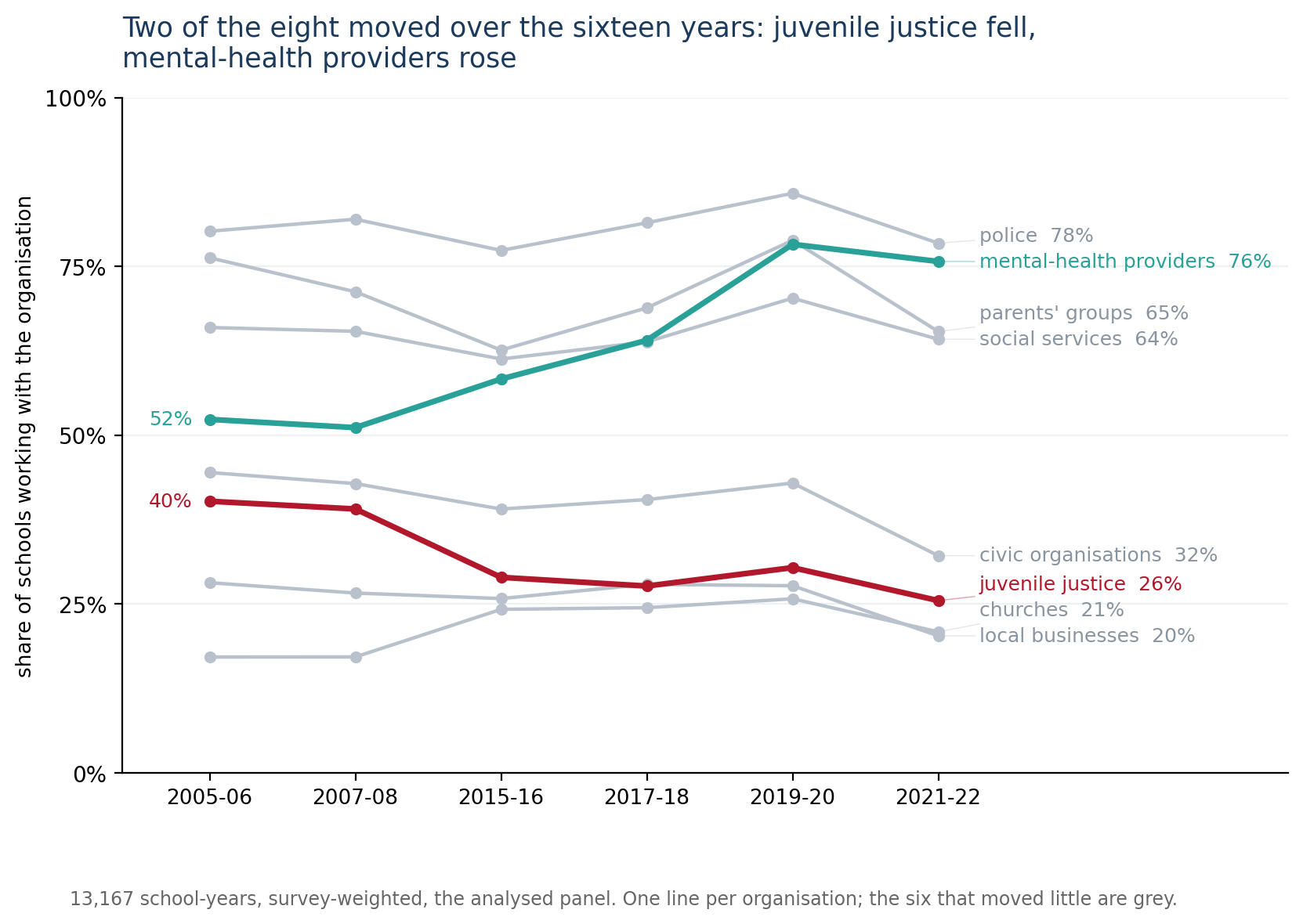
Table 20. Share of schools working with juvenile justice agencies and with mental-health providers, by survey and by the crime level the principal reportssource table 11
| 2005-06 | 2007-08 | 2015-16 | 2017-18 | 2019-20 | 2021-22 | Change | |
|---|---|---|---|---|---|---|---|
| Mental-health provider | |||||||
| High-crime areas | 69% | 69% | 75% | 78% | 87% | 71% | +2 pts |
| Moderate | 57% | 54% | 67% | 71% | 83% | 80% | +23 pts |
| Low-crime areas | 53% | 52% | 58% | 64% | 78% | 78% | +25 pts |
| Juvenile justice | |||||||
| High-crime areas | 47% | 36% | 20% | 33% | 20% | 21% | -25 pts |
| Moderate | 42% | 43% | 36% | 29% | 33% | 21% | -21 pts |
| Low-crime areas | 42% | 41% | 29% | 28% | 31% | 27% | -14 pts |
Note: Survey-weighted shares, n = 12,691. Crime level is the principal's description of the area. The two rows that changed over the period are shown; the other five organizations barely changed. On mental health, high-crime schools led low-crime schools by 16 points in 2005-06 and low-crime schools led by 7 points in 2021-22. Between 106 and 144 schools report a high level of crime in any one wave, so a single cell carries a standard error of roughly four points and the wave-to-wave movement in that row should not be read closely. Interacting the crime measure with time, the association with the count of organizations falls across the six waves by -0.134 (p = 0.013). The fall sits in the pandemic year, not in a gradual narrowing: estimated without 2021-22 it is -0.039 (p = 0.46), and on the four pre-pandemic waves -0.010 (p = 0.85). So the convergence in the levels shown above does not appear as a downward trend in the association before the closures. Taken one organization at a time the trend does not separate from zero either, at p = 0.11 and p = 0.12. ***p < 0.001, **p < 0.01, *p < 0.05.
The change did not happen evenly everywhere. Split the two organizations that changed by the crime level the principal reports and the shift shows up in both, running in opposite directions. Juvenile justice fell further in the schools whose principals call the area high-crime, by 25 points against 14 in the low-crime schools. Mental-health providers rose further in the low-crime schools, by 25 points against 2 in the high-crime schools, where they had been more common at the start.
Could it be the other way round?
So far this reads one way. A principal thinks the area is rough, and the school works with more organizations.
But maybe it works the other way. Maybe the school already works with a lot of organizations. They tell the principal the area is rough. And that is why the principal says so.
Here is how to check.
If partners were doing the telling, it would be the crime ones doing it. The police and juvenile justice agencies are the ones who would talk to a principal about crime. So turn the question around. For each of the seven, ask which ones go with a rougher description.
The answer comes out backwards for that story. Schools that work with the police have principals who report less crime, at -0.145. The two tied most closely to a rough description are mental-health providers at +0.126 and churches at +0.123, with local businesses close behind at +0.117. Count only businesses and churches and it is still there, at +0.102. Churches and shops do not brief principals on crime.
There is a second check. The principal's answer lines up with measures no partner could have supplied: crimes actually recorded at the school, how much bullying staff report, how few parents turn up. Those come from the school, not from the people it works with. In counts, a school whose principal calls the area high-crime records about 35 incidents a year, against about 16 where the principal calls it low-crime, and that holds among schools of the same size.
There is a third check. If having police in the building shaped how a principal saw the area, the sharper police questions would show it. The survey asks whether officers are there weekly, whether a written agreement covers their role and whether it covers discipline, and all three come out at nothing.
None of this settles the direction. Every survey is a fresh sample taken at one moment. No school is followed over time. The checks make the backwards story hard to hold. They do not prove the forwards one.
Table 21. Three checks on the direction: the crime level the principal reports against things it is not used to predict, the police relationship on every margin the survey records, and each of the seven organizations with the regression turned aroundsource table 15
| Coefficient | Clustered SE | p | |
|---|---|---|---|
| The reading against things that are not the outcome | |||
| Recorded incidents of crime and violence | +0.103*** | 0.011 | 0.000 |
| Reported bullying, harassment and verbal abuse | +0.154*** | 0.011 | 0.000 |
| How many parents turn up to school events | -0.185*** | 0.016 | 0.000 |
| The police relationship on every margin the survey records | |||
| Sworn officers at the school at least weekly (n = 8,293) | -0.010 | 0.007 | 0.153 |
| A written agreement defines the officers' role (n = 5,379) | +0.008 | 0.010 | 0.440 |
| That agreement covers student discipline (n = 2,780) | +0.013 | 0.010 | 0.183 |
| Each tie against the reading, if the arrow ran the other way | |||
| Civic organizations (community) | +0.049* | 0.022 | 0.028 |
| Local businesses (community) | +0.117*** | 0.032 | 0.000 |
| Churches (community) | +0.123*** | 0.031 | 0.000 |
| Social services (government) | +0.099*** | 0.025 | 0.000 |
| Mental-health providers (government) | +0.126*** | 0.029 | 0.000 |
| Juvenile justice (government) | +0.054* | 0.027 | 0.049 |
| Police (government) | -0.145*** | 0.042 | 0.001 |
| A count of businesses and churches only | +0.102*** | 0.022 | 0.000 |
Note: n = 12,691, except the parent-turnout row, which uses the 8,425 school-years in the four waves carrying those items. Survey-weighted, standard errors clustered on the sampling stratum within wave. The top panel asks whether the principal's reading tracks anything beyond the ties it is used to predict. The bottom panel reverses the regression: if a school came to describe its area as rougher because its partners told it so, the partners with a crime remit would be the ones going with a higher reading. The middle panel gives the police relationship on the margins the survey records beyond the tie itself, carried from 2015-16 on; the agreement rows apply only to schools with officers, and the discipline row only to those with an agreement, which is why their samples shrink. ***p < 0.001, **p < 0.01, *p < 0.05.
Table 22. The crime level the principal reports against what the school itself records
| The principal calls the area | School-years | Incidents recorded | Reported to police | Violent incidents | Any serious violent incident | Weapon disciplinary actions | Bullying at least weekly |
|---|---|---|---|---|---|---|---|
| Low crime | 9,488 | 16.3 | 5.4 | 10.7 | 18% | 0.5 | 16% |
| Moderate crime | 2,460 | 26.6 | 8.7 | 19.4 | 24% | 1.2 | 21% |
| High crime | 743 | 34.5 | 9.2 | 26.1 | 27% | 1.5 | 27% |
| Incidents recorded, within one enrollment band | |||||||
| Enrollment under 300: low, moderate, high | 1,458 | 7.5, 10.1, 21.3 | high 2.9 times low | ||||
| Enrollment 300 to 499: low, moderate, high | 2,612 | 10.1, 17.4, 20.2 | high 2.0 times low | ||||
| Enrollment 500 to 999: low, moderate, high | 5,057 | 17.9, 28.4, 40.5 | high 2.3 times low | ||||
| Enrollment 1,000 or more: low, moderate, high | 3,564 | 48.1, 71.7, 82.9 | high 1.7 times low |
Note: Survey-weighted means per school, and shares, on the analyzed panel. The counts are NCES's own, derived from the incident battery the school completes; the principal's reading is question 50, the crime level in the area where the school is located. Schools whose principals call the area high-crime record 2.1 times as many incidents as those whose principals call it low-crime, and the gradient holds inside every enrollment band. Violent and serious violent incidents are absent from the 2021-22 file and disciplinary actions start in 2007-08, so those columns run on fewer years. As a rank correlation, weighted, the reading goes with incidents recorded at 0.17, with violent incidents at 0.19 and with reported trouble at 0.19: the averages double while most schools in every category record few incidents, so the reading separates groups of schools more sharply than it ranks single ones. All of these come from the school on the same questionnaire; the public files carry no geography that would allow a check against crime recorded outside it.